On September 17, 2018, the King County council voted
5-4
to allow for a
new funding agreement between King County and sports stadiums such as
Safeco Field. There have
already
been challenges
to the legislation and it may appear as a
petition
on the ballot soon.
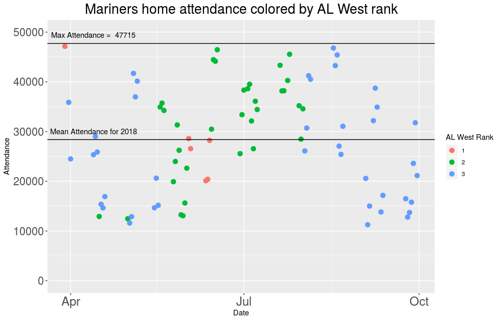
The 2018 season was unusually successful for the Mariners, and while
they are again sitting out the Playoffs this season I did wonder what
attendance looked like this year.
I added two lines to this plot, one for maximum attendance (currently
47,715 according to
Wikipedia)
and one for mean attendance which was 28,389 this year. This means that
we have a
stadium that is on average about 60% full for any game for a team that
competed for a
Playoff spot until the very end of the
season.
Is that really the best use of this money?
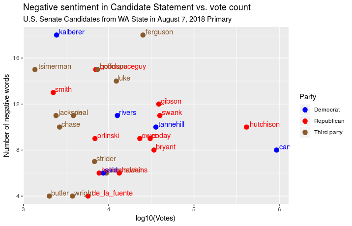
The 2018 Washington State
Primary was held on
August 7, 2018. As a
registered voter in Washington State I am mailed a Voter’s Information
Pamphlet
which lists the candidates and a Candidate
Statement (provided by the candidate) for each office. The Candidate
Statement is where the candidate is allowed to write anything they want
as long as its under 300 words. I was curious if there was any
relationship between the sentiment of a candidate’s Statement and the
number of votes
that candidate received.
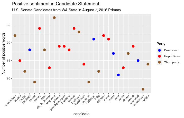
I conducted my analysis using sentiment analysis which groups words
together based on
pre-defined lists of words that are members of that group. There are
many word groups to choose from such as “joy” and “trust” but for this
analysis I just looked at “positive” and “negative” words (as classified
by NRC).
Although there were many different offices up for election in this Primary,
the U.S. Senate race had 29 candidates which made for a very rich
dataset. Washington State uses a Top-Two
Primary
which allows for easy comparison across political parties.
There are many factors deliberately ignored by this analysis such as
PVI,
incumbency, fundraising, political party and candidate issues. However I thought
text mining could
be an interesting way to analyze these candidates in a slightly
different manner.
First I just plotted the number of positive words in the Candidate
Statement for each candidate:
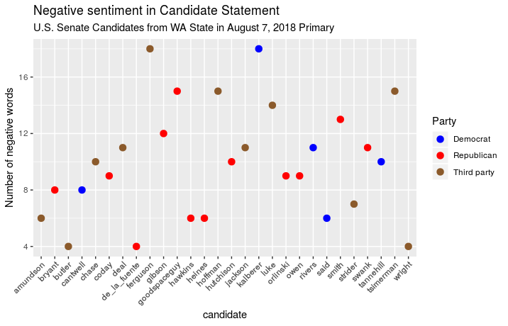
Then I repeated with the number of negative words in the Candidate
Statement for each candidate:
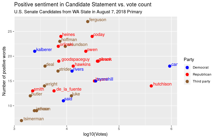
Next I looked at the number of positive words in the Candidate Statement
by candidate versus the number of votes that candidate received. Because
of the strength of the Democratic incumbent candidate Maria
Cantwell and the Republican
establishment candidate Susan
Hutchison I had to
log-transform the vote counts because these two candidates got so much of
the total vote.
Then I repeated this analysis by looking at the negative word count for
each candidate versus the total log-transformed vote count:
While I don’t think this will lead to any novel political insights, I
do think its an interesting way to look at candidates. Full code
including individual candidate statements available
here
Like many other metropolitan areas, Seattle is currently dealing with a
serious housing shortage. Recently, there have been some good articles
(here
and
here)
about converting public golf
courses into housing. It is an interesting concept and certainly should
be discussed, however one aspect I feel is being overlooked in this
debate
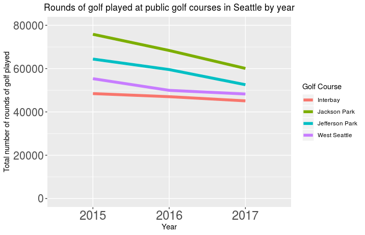
is how popular are these golf courses anyways? According to Bloomberg
News, there is declining interest in golf
nationwide,
is this happening in
Seattle?
The City of Seattle is somewhat
aware of this issue and is at least discussing
options
for the golf courses. I filed a Public Records
Request act
with the City of Seattle and they sent me data on the rounds of golf
played for
the past three years.
Unfortunately the city only provided the count data for number of
rounds of golf played per year so I cannot look at more granular trends.
However, I can plot the counts on an annual basis.
It will be interesting to see if this debate both on converting public
golf
courses to housing goes anywhere both in Seattle and other major cities.
I don’t have a horse in this
particular race, I live near the Jefferson
Park course and I
really appreciate the large
expanse of green it provides however I am acutely aware of the need for
more housing within Seattle city limits.
Interested in taking a look? I put the full data I got from the city
here.
One of the things people consistently tell me when they are
considering buying or renting a home in a new location is
that they want to move somewhere with “good schools.” This always makes
me wonder how we quantify what schools are
considered “good”? To start you might look for information on school
reputations or performance using local school data fact sheets from
realtors or apartment managers or, more likely, by searching ranking and
review sites such as
Niche.
This approach is generally fine but it assumes that you are only
interested in a specific neighborhood which may be difficult to achieve
right now in most major cities across the US and especially in
Seattle.
What if instead we looked at all the neighborhood school ratings in a
city simultaneously? This would
allow the reader to spot trends and make visual comparisons as well
as possibly identify overperforming schools in unexpected areas.
Fortunately, Seattle Public Schools (SPS) provides quite a lot of
data
about their schools which makes this easy to visualize.
Setup
For this analysis I just the SPS data for the 2016-17 school
year.
I focused solely on elementary school data for the 2016-17
school year. I used the SPS district boundary map for all public elementary
schools in the City of Seattle and ignored any magnet or alternative
elementary schools.
Rankings
Initially I focused on three questions:
What school has the best student/teacher ratio?
What school reports the best attendance?
What schools are best for reading and math?
I took the SPS data for student/teacher ratio, attendance rate, and reading and math
proficiency scores for each school and calculated their rank
within the city to make this table. Click on the category name to sort
by that category.
School Name
Attendance Rank
Student/Teacher Ratio Rank
Grade 3 Math Rank
Grade
3 Reading Rank
Adams
12
53
29
21
Alki
20
35
12
15
Arbor Heights
21
31
45
33
Gatzert
42
4
49
56
Beacon Hill Int’l
1
32.50
30
37
B.F. Day
16
43
25
23
Broadview-Thomson K-8
49
2
46
45
Bryant
6
55
3
4
Cascadia
2
59
1
1
Catharine Blaine K-8
38
15
6
13
Concord Int’l
44
22
59
60
Bagley
10
20
24
19
Dearborn Park Int’l
61
61
61
61
Dunlap
43
5
56
55
Emerson
58
14
43
53
Fairmount Park
22
47
2
3
Coe
9
48
10
9
Gatewood
35
26
33
40
Genesee Hill
24
50
16
20
Graham Hill
39
10
55
49
Green Lake
31
37
26
28
Greenwood
15
54
20
17
Hawthorne
46
16
48
41
Highland Park
48
6
57
50
Hay
8
38
19
10
John Muir
23
25
52
48
John Rogers
33
24
34
34
Kimball
30
32.50
40
36
Lafayette
29
44
27
25
Laurelhurst
34
49
15
24
Lawton
26
42
4
6
Leschi
53
36
37
44
Lowell
60
3
58
54
Loyal Heights
17
58
5
7
Madrona
52
1
47
43
Maple
19
28
31
32
MLK Jr.
45
8
54
58
McDonald International
7
30
23
2
McGilvra
25
40
14
11
Montlake
37
51
9
16
North Beach
14
46
13
12
Northgate
51
11
50
51
Olympic Hills
41
34
21
30
Olympic View
27
56
32
29
Queen Anne
28
57
28
22
Rainier View
55
21
18
26
Roxhill
56
13
53
57
Sacajawea
36
7
42
42
Sand Point
47
27
39
35
Sanislo
57
12
60
59
Stevens
32
29
35
31
Thornton Creek
18
17
41
38
Thurgood Marshall
5
39
8
18
Van Asselt
59
9
51
52
Viewlands
40
19
44
47
View Ridge
3
52
11
5
Wedgwood
11
41
7
14
West Seattle Elem
54
23
38
46
West Woodland
13
45
17
8
Whittier
4
60
22
27
Wing Luke
50
18
36
39
Schmitz Park
62
62
62
62
What jumps out at me most is that no particular school consistently
out-performs the others, which can make it challenging to decide what
to prioritize when choosing a school.
Student/Teacher ratio
Each school reports the number of enrolled students and the number of
teachers which I simply used to calculate a ratio.
Click on an attendance area for the exact percentage.
Attendance
I was initially interested in student attendance data, but the elementary
school with the
lowest daily attendance was Lowell Elementary with an attendance rate of
89%. Every other school reported an attendance rate at or
above 95% which did not make for a very interesting map. I later learned
that Washington State has a compulsory
attendance law
which likely affected these numbers.
Reading proficiency
I was interested in looking at district-wide third grade reading achievement scores district-wide
for 3rd
graders as measured by the Washington State proficiency
test. I
chose third grade because that is the first year a Washington State standardized test is
administered for reading.
Click on an attendance area for the exact percentage.
Click on an attendance area for the exact percentage.
Family engagement
SPS provides a parent survey with a variety of questions evaluating
parent enthusiasm and approval of Seattle schools. These survey results are not published, so I looked at how many families
completed these surveys for the 2016-17 school year.
Click on an attendance area for the exact percentage.
Even the school with the most responses reported that only 49.1% of families responded to the
survey which to me means that most families are satisfied with
their school but neither especially excited or disappointed by their school experiences.
tl;dr Choosing a school is hard but ultimately it comes down to how
satisfied the parents or guardians are with the school. Schools report
on a wide array of metrics about student performance,
but performance is often an issue of secondary importance when
compared to parents’ overall perception of the school quality.
Remember this map that Facebook created of friend connections back in
2011?
I thought it was pretty cool back then and I still
think its pretty cool. I wanted to make a similar map but was not sure
where to start. I could have done a similar visualization however I
recently quit
Facebook so I can no longer export all my friend’s data to use for
making maps. My next thought was visualizing travel routes such as flight information. I am trying to
reduce my carbon footprint which meant I only flew five times in 2017
and have flown exactly zero times so far in 2018. Then I thought, you
know who does
fly alot? The Seattle Mariners.
First step was to collect all the Mariners game data, fortunately
Baseball Reference has all that data in an easily accessible HTML
table.
Next step was to geolocate all the stadiums which can be a bit tedious.
Fortunately GitHub user
the55 created a nice JSON file of all the
stadiums and put it as a
gist. I was able to use an R
library called
geosphere for
using the Haversine
formula to calculate
the distance between two stadiums.
My initial attempt here:
In order to make the image look similar to the Facebook connection map,
I ended up using this Flowing Data
post
quite a bit to figure out how to
add the lines and change the background color:
Finally because there were so many trips from Seattle to American League
West opponents that I ended up adding a bit of noise or
jitter to the stadium locations
to make the flight paths not perfectly overlap each other.
Looking back at this 2017 reminded me the Mariners finished 78-84 in
2017, here’s hoping to a better season in 2018!
If interested, I put all the code for this analysis
here
This is my second post looking at the data from the 2017-18 Washington
State Legislative Session. the first part of this blog can be
read
here
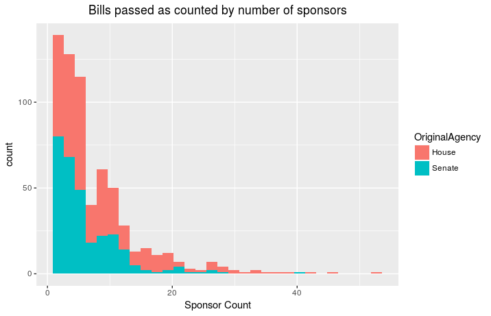
After some time looking at different bills that did pass, I started to
wonder if a bill
was more likely to pass if it had more sponsors. First I took the 647
bills passed by the Legislation and signed into law by Governor and
looked up how many co-sponsors each bill had:
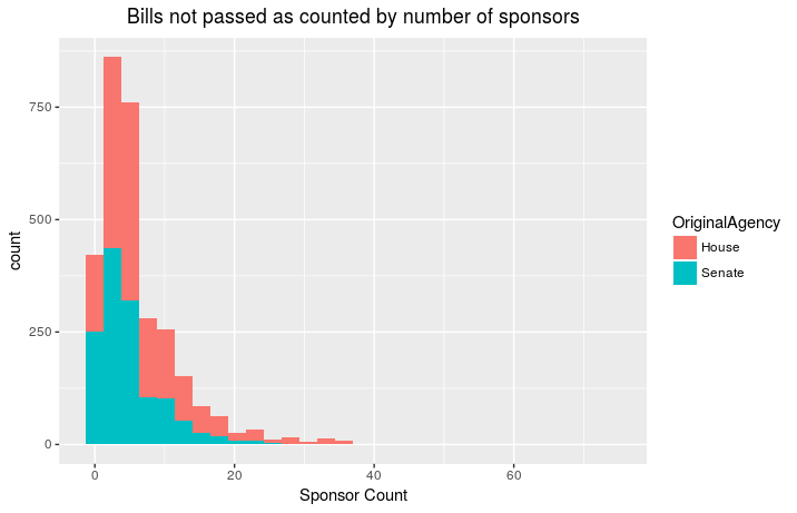
Then I I took every bill that was introduced but did not become
law and counted up the sponsors for these:
So it appears that the number of sponsors is not particulary predictive
for a bill becoming law. The three bills introduced in the Senate with
the highest number of Sponsors were:
Creating Washington state aviation special license plates.
In November 2017, Manka Dhingra won a special election and the
Washington State Senate
flipped from Republican held to Democrat held. Initially I wanted to
focus on the number of bills passed by a Republican held Senate versus a
Democrat held Senate but there were too many extraneous variables such
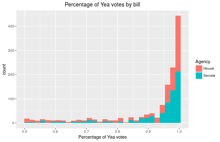
as passing a budget and a shorter session in 2018. Instead, I decided to
focus on the number of Yea votes by bill
Many of the bills passed were with almost overwhelming support, which is
refreshing to see that there is quite a bit of bipartisanship in
Washington State in 2018.
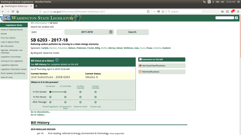
In his 2018 State of the State
speech,
Washington State Governor Jay Inslee
made a passioned appeal for a carbon tax and proposed one in Washington
State Senate bill
6203.
Because of this, I paid more attention to the
activities of the Washington State Legislature than I ever had before
and I found it fascinating.
First off, lets start with the website for the state Legislature. Here
is a screenshot of the
Washington State Legislature page for SB 6203 which is the bill I was
most interested in:
The website is very resource dense and well worth time exploring when
the Legislature is in session. Every piece of proposed legislation
shows the same amount of information and allows you to easily find and
contact your legislators about a particular bill if interested. The site
also has livestreams of committee
hearings
and displays vote
counts on bills in almost
real time as the votes are tallied on both the
Senate and the House floor.
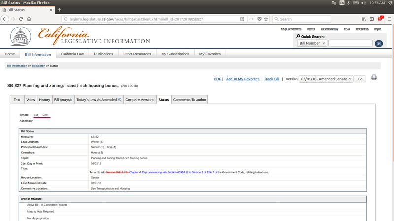
Is Washington State unique in this regard? Of course not, here is a
screen shot for an interesting bill in Legislature for the State of
California.
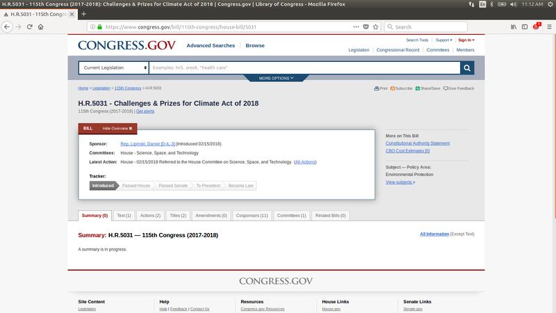
Finally here is a screenshot of a House bill on the United States
Congress website
Does ease of use of the website increase participation in the civic
process at the state level? That is a difficult question to answer but
personally I am glad I get to use the Washington State one instead of
the California State Legislature webpage.
The 2017-18 Washington State Legislative Session ended on March 8,
2018
and
Governor Inslee then had 21 days to sign bills into law or veto them.
The conclusion of the 2017-18 Session made me wonder what happened to
those bills that were introduced and how many of them actually became
law.
In addition to a great website, the Washington State
Legislature also has an excellent set of Web
Services that allow for
programmatically
capturing metrics and data about activities in the state
legislation. One way to easily visualize this is with a Sankey
Diagram (no relation to
this Sankey though).
Here is a smaller image of the diagram with a larger version
here
Code to generate this figure available on my GitHub repo
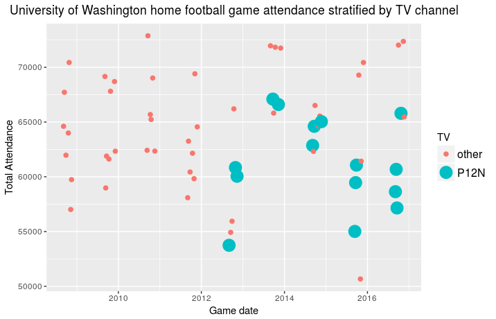
Following up on my earlier
post,
how much has the Pac-12 Network affected game attendance? I updated my previous data set to include the past two seasons so as to include 2008-2017 data. I relied on home game
attendance as reported by Wikipedia and also used Wikipedia to determine what TV network broadcast each home game. In an ideal world I would be able to make better comparisons using the Nielsen rating
for each game however my guess is that data does not come as cheap or as
easily as data from Wikipedia. For the purposes of this analysis I am
neglecting various other factors in this anaysis
such as time at kickoff, game day temperature, opponent, ranking of UW,
ranking of opponent, etc… the list goes on and on. My main intention
was
to simply show home game attendance versus TV network for all games:
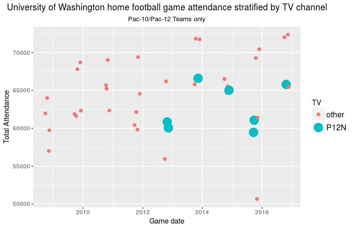
And attendance for Pac-12 only opponents versus TV network:
Based on the available data it appears that attendance during home games
has
been influenced and possibly decreased by the Pac-12 Network but it is
difficult to say for sure while ignoring so many external factors. With
a significant budget deficit still a major
issue,
one can only hope that losses from game day ticket sales are made up for
with Pac-12 Network advertising revenue.
With WSU beating
Oregon and
UW beating UC
Berkeley,
the State of Washington is poised to have two football teams in the top
ten of NCAA Division I football rankings. Naturally this got me
thinking, how often does this happen and how many states have had this
same achievement?
To answer this I used the weekly results of Associated Press
poll which started in 1936 and
thanks to our good friends at Wikipedia,
I was able to get AP Poll results for every week.
I found that 25 states had at least one week where two teams from that
state were in the AP Poll. However, the more I thought about it the more
I realized this was slightly biased because some states might only have
one team (i.e. Wyoming) while other states might have two Division I
teams that are never both great at the same time (i.e. Montana). I
tightened down my restrictions a bit and only looked at the top 10 teams
from each AP Poll.
Surprisingly, of the 25 states with at least two teams in the AP top 25
Poll,
21 of those states had a week with at least two teams from that state in the AP top 10.
I made a summary table with the most recent year each state achieved
this distinction listed:
I wanted to revist my previous
post
continuing to look at using linear
regression for determining the best
episodes of a TV show to watch. I started to think about how to look at
this data for multiple TV shows. Performing a linear regression on show
rating by episode number within a season quickly allows us to determine
the maximum and minimum residual for all the show episodes. I took this
a step further and
calculated which episode of the show it was. For example, here are all
the episodes with residual value for that particular show Master of
None:
Season
Episode
Name
Residual
count
appearance
1
1
Plan B
-0.28
1
0.05
1
2
Parents
0.21
2
0.1
1
3
Hot Ticket
0.01
3
0.15
1
4
Indians on TV
0.21
4
0.2
1
5
The Other Man
-0.09
5
0.25
1
6
Nashville
0.31
6
0.3
1
7
Ladies and Gentlemen
-0.39
7
0.35
1
8
Old People
-0.09
8
0.4
1
9
Mornings
0.11
9
0.45
1
10
Finale
0.01
10
0.5
2
1
The Thief
0.44
11
0.55
2
2
Le Nozze
-0.36
12
0.6
2
3
Religion
-0.27
13
0.65
2
4
First Date
0.13
14
0.7
2
5
The Dinner Party
0.02
15
0.75
2
6
New York, I Love You
0.42
16
0.8
2
7
Door #3
-0.89
17
0.85
2
8
Thanksgiving
0.31
18
0.9
2
9
Amarsi Un Po
0.30
19
0.95
2
10
Buona Notte
-0.10
20
1
We can see that the episode with the highest residual is S2E1 “The
Thief” and the episode with the lowest residual is S2E7 “Door #3”. For
every TV show I took all the episodes and calculated their order as a percent of
the total number of episodes - for example the pilot episode would be 0.0 and the
series
finale would be 1.0 to generate an index. I then took the
maximum and minimum residual values for each show and plotted them
against that episode. For example here is a plot of just Master of None:
To obtain data on as many shows as I could I used this IMDb
list
of shows with over 5000 votes and selected the first 1200 shows as a
dataset. I then reused the OMDb API as I did before. I then calculated the same values as I did for Master of None
above and plotted them in a similar manner (use the mouseover for more
information on each point):
Two things immediately jump out at me:
The density of points right around the zero line shows that linear
regression is a pretty good metric to use for this type of analysis and
that most people rate the show generally in line with the overall trend
for that particular season.
There seems to be a tendancy for people to really love or really hate
the series finale of TV shows and this shows up by the sheer number of
points at 1. Possibly this is people expressing their overall view of
the show as a whole or maybe people really were really happy or unhappy
with the series finale.