Zach Stednick

Open Street Map (OSM) is, simply put, a freely available and editable map of the world. I have been interested in improving the availability of boundaries in Seattle and wanted to add park boundaries to this list as well. It was easy to look up boundaries on OSM, for example Salmon Bay Park shows the various nodes that make up its boundaries. But I had struggled with how to automate this search since at last count Seattle had over 400 parks. After months of struggling with the OSM API, I fortuitously stumbed across the following tweet:

Two map data posts: Historic map warping for @somethingmodern http://t.co/7POw8PNBXI Data from OSM for @alignedleft http://t.co/DqxAuyPunh

— Michal Migurski (@michalmigurski) August 15, 2015

This tweet lead me to Mapzen which provides a service called Metro Extracts which provides datasets from OSM on a weekly basis. I downloaded the OSM2PGSQL GeoJSON file for Seattle which provided me files for Line, Point, and Polygon geometries. I then used ogr2ogr to filter for parks only with the command

ogr2ogr select 'osm_id, name, geometry' where "leisure = 'park'"

This produced a GeoJSON file that looked like this:

Obviously, more filtering needed to be done. Since many of these parks were not in Seattle, I used the Nominatim API to search for each park based on the OSM ID number. For example, the above mentioned park Salmon Bay Park returns a nicely formatted XML file which I just filtered based on city.

Even after this there were still parks that were wrongly labelled as being in Seattle. I loaded the file into R and subset based on OSM ID and then used rgdal to write the final result out as a GeoJSON file.

The take home lesson for me is that OSM is an excellent service but as with any publically annotated dataset be prepared to invest some time into cleaning and validating the data.

I have been tracking restaurant openings via the City of Seattle Business Finder since the beginning of this year and am reporting those changes at Seattle Restaurant Changes. Recently I put up a heatmap showing changes by neighborhood. This heatmap shows a current snaphot of the changes which made me curious about changes by restaurant type over the course of the year.

A few notes:

• The City of Seattle uses North American Industry Classification System codes (NAICS) to track restaurants. I then use the date of permit issuance as a proxy for a restaurant opening and date of permit revocation as a proxy for closing.

• A Full Service Restaurant as defined by NAICS is “establishments primarily engaged in providing food services to patrons who order and are served while seated (i.e., waiter/waitress service) and pay after eating”

• I realized that not that many breweries would be opening up but who doesn’t want more breweries in town?

• I was not expecting Full Service Restaurants to take off as much as they did, especially since Limited Service Restaurants seem to be declining.

I will try to post another update on this in December, that is unless I decide to open up a food truck of my own.

I was listening to the Jonah Keri podcast and he and Ben Gibbard were talking about the Mariners, specifically Felix Hernandez. One of the points Gibbard made was that Hernandez is so outstanding that he will be remembered and that people should try to see him pitch in person. This made me wonder, did Felix Hernandez have an impact on home ticket sales for the Mariners in 2014?

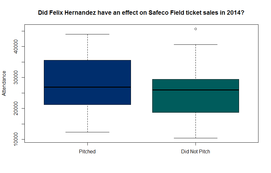
I was able to get all the data from some of the nicely formatted box score data that MLB provides. I initially tried to look at the data over the course of the year but attendance was so variable (which made for an extremely confusing plot) that I just ended up making a box and whiskers plot and ignored the date element:

Conclusion: Hernandez was not that strong of a driver of ticket sales which is great news if you are hoping to see him pitching in person.

Seattle construction is currently booming and I was interested in how that reflected in the local restaurant scene. There are many food blogs and local news sites that cover openings and closings, but I found it too difficult to parse these in a regular manner. Fortunately I was able to use data from the City of Seattle business finder and used the restaurant classification or NAICS code as a proxy. Using the data in this manner makes an assumption that a restaurant will no longer have a business licence after it closes. I’m not sure how accurate this is but I figured it was as accurate as I could get short of hiring people on Mechanical Turk to phone every restaurant every week and ask if the restaurant is still open. To map each restaurant to a particular neighborhood, I used geolocation to map license address returned by the City of Seattle business finder. Obviously that does not work as well for Mobile Food Services (i.e. food trucks) but it still allows for an interesting comparison. This data is plotted at Seattle Restaurant Changes.

I initially attempted to scrape data from The Stranger but after finding the City of Seattle site I just used BeautifulSoup for the scraping. I would not have been able to do much more beyond that state if it had not been for Nathan Yau’s excellent tutorial on making maps with category filters. I was able to get a state level shapefile for Washington state from Zillow and then reduce that to just Seattle neighborhoods using R’s sp package. Full code posted on github

After a year on Fitbit, I figured it might be time to take a look at the data that I have been generating. Unfortunately, Fitbit makes you sign up for Premium which charges you $50 per year to export your data. Fortunately, Cory Nissen has created an excellent R package for doing just this. The package simply uses a POST request handled by Hadley’s httr library to generate a cookie and then parses the returned JSP results to return a nice data.frame.

Anyways, onto the data.

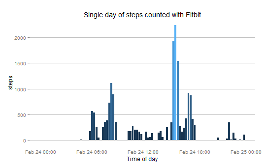
The first command I tried was the get_15_min_data() for parsing step data in 15 minute increments. I figured that looking at yesterday’s data would be granular enough to get a good feel for the data.

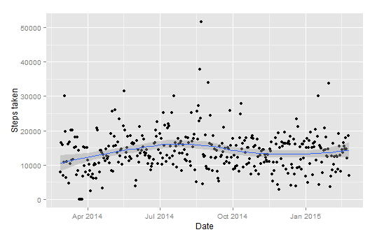
I then plotted number of steps taken per day, with a smoothing function overlaid:

I had a mean step count of 13935 for the past year. This data is more interesting to look at as more of an overall trend. There definitely a seasonal trend in the summer which makes sense. I can also see the signatures of when I went on a four day backpacking trip in August and when I broke two ribs and was confined to the couch for four days in mid-March.

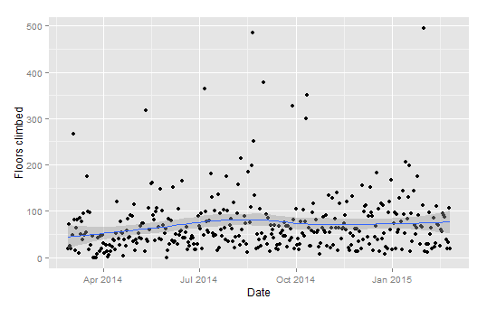
Since I have a Fitbit one, I can also measure floors climbed.

My mean number of floors climbed is 69.62 which seems absurdly high. My desk is on the fourth floor of my building and I usually take the stairs but not sure that is enough to fully explain why these counts are so high.

Still, it is pretty interesting to look at this data outside of the Fitbit interface and I would highly recommend checking out Cory’s github repo

Also, speaking of github, for those of you who regularly follow this blog (hi, Mom!) I have moved away from making a new gist every time to simply having a standalone repo

Last year, among other personal data, I tracked every bar I went to and every mile I ran. Naturally my first question is do I run enough to offset the amount of beer I am drinking (at bars)?

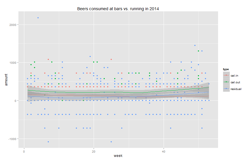
First we define some units. According to this Runner’s World calculator, at 8:45 minute/mile for my weight I am burning 145 calories. Google says the amount of calories in a pint of beer is about 180. Since I usually average about two beers each time I go to a bar, that simplifies the calculations. Over the course of the year, how often was I above or below the residual? To answer this, I used R and finally got around to trying tidyr which is pretty slick.

I thougth a lot about how to determine the residual but eventually settled on calories out - calories in because I felt this method made the best visualization. As you can see around week 30, I started to run more and did a better job at offsetting my beer consumption. Obviously this is an overly simplistic view of my caloric expenditure but shows some of the interesting insights that can be gained from personal data.

As always, all code and data is in this github gist

I recently read an interesting blog post where the author examined their books rated on Goodreads and summarizing interesting trends. I decided to do a similar analysis even though I use LibraryThing instead.

LibraryThing has a nice option to allow to to export your data in a variety of formats. Since I write R code to parse CSV files everyday I thought I would do something different and parse a JSON file with python.

I have been on LibraryThing since 2007 and the first question I was interested in was have my average ratings changed over time? I calculated the mean for each book by year:

While uninteresting, this makes a lot of sense - if I am reading a book that I do not enjoy, I will usually bail on it which tends to bias my ratings upward. Over time, there have been a few notable exceptions.

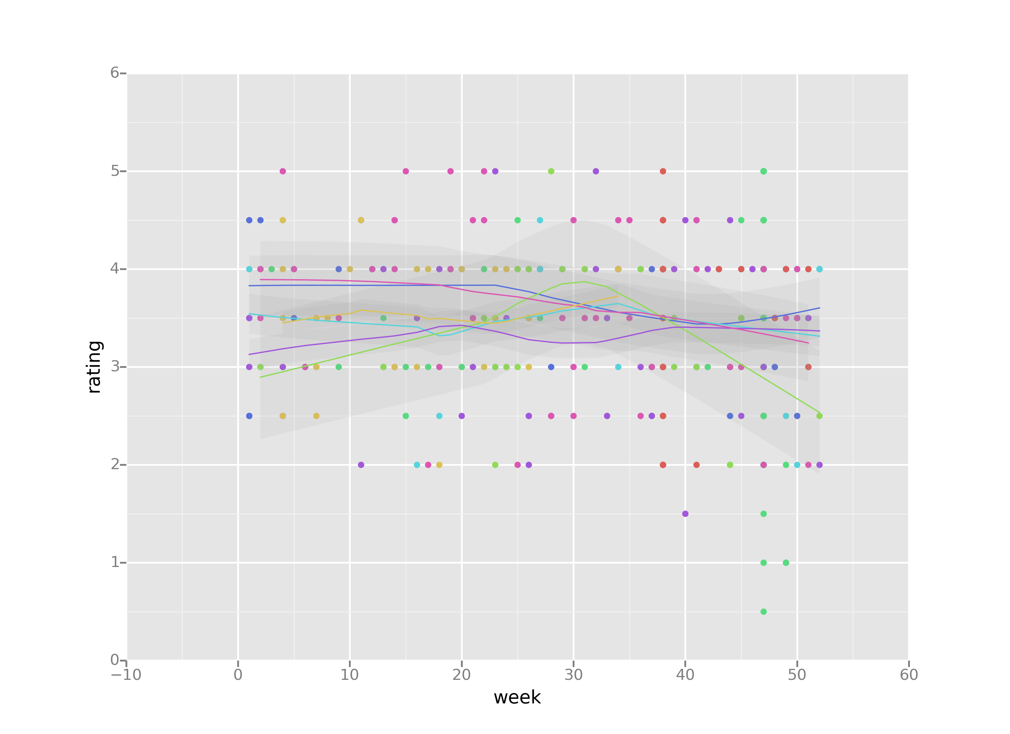
One of the other interesting analyses in the blog post was examining how the reviewer’s ratings have changed based on the month of the year. I wanted to make a similar plot using R’s ggplot2 however since I was writing this in python I was largely limited to matplotlib. Fortunately, many people have struggled with this issue and the fine folks at yhat have ported ggplot2 over to python. With this library I was able to use geom_smooth to produce the following plot showing rating trends by week.

I tried to figure out why my legend never showed up but I figured that since most of the trend lines were pretty much the same anyways that the plot was fine without a legend. It appears that I get in most of my good reviews early in the year and am harsher later in the year.

The last figure in the blog post compares the writer’s review scores to the Goodreads consensus score. I attempted to replicate this but ran into more trouble than it was worth to extract that data from LibraryThing so I abandoned that analysis.

If interested, I put my python code in a GitHub gist.

As someone who puts out writings out publically, I am naturally curious who (if anyone) is actually reading what I write. To answer this I developed a simple webstat calculator using R. I realize there are many options out there for tracking visits but to paraphrase my friend Andy, when has using standard libraries lead to anything cool?.

My main interests in this project is to answer two questions:

1. Are people visting this site?

2. Where are they visting from?

I don’t really care about things like bounce rate or type of device used to access the site. Not having to worry about either of these issues helps cut down on the complexity. I run this site on an Apache server and use a standard log output to write my logfile: LogFormat "%v:%p %h %l %u %t \"%r\" %>s %O \"%{Referer}i\" \"%{User-Agent}i\"

I made a small R script that uses knitr to output plots to HTML for ease in viewing. I wrote a shell script that uses the excellent little r to perform the commands. I run the shell script daily as a cron job and only look back at the past week’s worth of data. Since this blog is served on github pages, it can be difficult to see page views so I use images loaded as a proxy.

Here are some example plots of recent visitors:

And then another plot of visitor locations:

That outlier from Brazil is likely a Google bot crawling the site; better detection and removal of bot traffic from the final output is on the TODO list. All of the code (minus the shell script) lives on github

I recently became aware of the efforts of Linnea Westerlind who made a goal to visit every park in Seattle and documented her efforts here. I thought this was pretty neat so I looked up the list of City of Seattle Parks which currently lists 419 parks. The definitions for a park are hard to determine and this list ends up with some oddball parks such as Crescent Place. Still I think it is an interesting way to learn more about where you live wherever that may be. I have currently visited 118/419 parkswhich is about 28%, not bad. Not sure if I will be able to reach them faster than the 4 years it took Westerlind but maybe I should just focus on the journey instead.

LEGO recently introduced a new LEGO set called Research Institute which featured three female scientists. Since my wife is also a female scientist, I tried to order one from the LEGO website only to learn that they had sold out in less than a day. I then wrote an email complaining about this to LEGO who responded by sending me an apology note and a catalog.

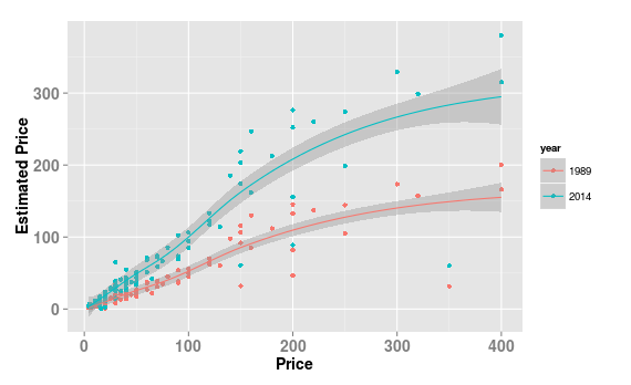
I grew up playing with LEGO sets, hard to avoid when you were named Zach and commercials like this dominated the airwaves. Anyways, when I was a kid my dad once mentioned to me that a good rule of thumb for determining the price of a LEGO set was to estimate each brick costing about 10 cents. This new catalog made me wonder if this was still true. I copied all the model numbers as well as the number of pieces and the prices. I was also curious in how true this trend was when adjusted for inflation so I used the CPI Inflation calculator from US Bureau of Labor Statistics which showed that $0.10 in 1989 had the same buying power as $0.19 in 2014. Ideally I could have found a catalog from 1989 but I don’t remember any back then and I probably would have cut it up to put pictures in my locker or something like that. I used R to plot both of these trends and it appears that my dad’s estimate still holds true for 2014.

A correlation calculation for all sets gives a value of 0.91 which means my dad had a pretty good estimate back in the day.

I also looked at the average price for each collection and found that almost all collections retained a high correlation between the estimated price and the actual price.

Raw data and code for this lives at this gist